字号与磅数

- 1 pt＝0.35146mm 约等于0.35mm

- 1mm约等于2.83pt

- 1英寸＝72pt

- 字高1厘米的字符，其磅数值大约为28.3Pt

- 3pt : 4px=1

中文字号	英文字号（磅）/pt	毫米/mm	像素/px
初号	42	14.82	56
小初	36	12.7	48
一号	26	9.17	34.7
小一	24	8.47	32
二号	22	7.76	29.3
小二	18	6.35	24
三号	16	5.64	21.3
小三	15	5.29	20
四号	14	4.94	18.7
小四	12	4.23	16
五号	10.5	3.7	14
小五	9	3.18	12
六号	7.5	2.56	10
小六	6.5	2.29	8.7
七号	5.5	1.94	7.3
八号	5	1.76	6.7

命题, 定理, 公理等使用区分

Proposition, 命题是一种要么为真要么为假的陈述。它通常被认为不如定理重要，但仍然很有趣和有用。与猜想不同，命题通常相对容易被证明或反驳
Theorem, 定理是一种重要而有意义的陈述，它已被证明是基于先前建立的陈述（例如其他定理、公理和引理）而为真。
Lemma, 引理是一种次要结果，其主要目的是帮助证明定理。它是证明更重要结果的垫脚石。
Corollary, 推论是从先前证明的定理中很容易得出的陈述。它通常是定理的直接结果，几乎不需要或根本不需要额外的证明
Conjecture, 猜想是基于某些证据或直觉提出但尚未被证明或反驳的陈述。它本质上是一种有根据的猜测，需要证明才能被接受为真。例如，著名的黎曼假设就是一个猜想，因为它尚未被证明
Axioms,是一种被视为不证自明的真理的陈述或命题，可作为进一步推理或论证的起点

行为决策理论中前景理论、失望理论和后悔理论

前景理论、失望理论和后悔理论都是行为决策理论的一部分，它们用不同的角度来分析人们在面对不确定性时的选择偏好和心理影响。

前景理论（Prospect theory）由卡内曼和特沃斯基于1979年提出，它认为人们的决策不是基于绝对的效用，而是基于相对的参照点。人们对收益和损失的敏感程度不同，通常对损失更加厌恶。人们在面对收益时倾向于风险规避，而在面对损失时倾向于风险寻求。
失望理论（Disappointment theory）由贝尔曼和拉皮德于1987年提出，它认为人们的决策不仅取决于结果的期望值，还取决于结果与期望的差距。如果结果低于期望，人们会感到失望；如果结果高于期望，人们会感到满意。失望和满意的程度与差距的大小成正比。
后悔理论（Regret theory）由贝尔、卢姆斯和萨格登于1982年提出，它认为人们的决策不只关心自己的结果，还会与其他可选方案的结果进行比较。如果发现其他方案的结果更好，人们会感到后悔；如果发现自己的方案的结果最好，人们会感到欣喜。后悔和欣喜的程度与结果的差异成正比。

一个Python画图的例子

在3d图中绘制多个线图

import matplotlib.pyplot as plt
from mpl_toolkits.mplot3d import axes3d
import numpy as np
x=np.linspace(0,20,40)
y_list=[1,3,5]
z=np.sin(x * 2 * np.pi) / 2 + 0.5
color_list=['red','tab:blue','tab:green']#颜色
font3 = {'family' : 'Arial',
    'weight' : 'normal',
    'size'   : 14,
    }
ax = plt.figure(facecolor='white').add_subplot(projection='3d')
#结合for循环绘制多张线图
for i in range(0,3,1):
    y=y_list[i]
    y=y*np.ones(40)#保证与x轴的点数一致，这一步非常重要
    ax.plot(x,y,z,linewidth=1,label='y='+str(y_list[i]),color=color_list[i])#绘图

# 图像的其他参数设置
ax.view_init(15, -20)#图形展示角度
ax.grid(False)#去掉网格
# ax.w_xaxis.set_pane_color((1.0, 1.0, 1.0, 1.0))#背景设置为白色
# ax.w_yaxis.set_pane_color((1.0, 1.0, 1.0, 1.0))
# ax.w_zaxis.set_pane_color((1.0, 1.0, 1.0, 1.0))
# ax.set_facecolor("white")
# # ax.patch.set_facecolor("gray")


ax.xaxis.pane.fill = False  # Disables the pane fill
ax.yaxis.pane.fill = False
ax.zaxis.pane.fill = False

ax.xaxis.pane.set_edgecolor('w')  # Sets the edge color to white
ax.yaxis.pane.set_edgecolor('w')
ax.zaxis.pane.set_edgecolor('w')



#坐标及坐标轴相关设置
ax.legend(frameon=False,fontsize='small',loc='center left') #设置图例及图中文本显示
ax.set_xlabel('x',font3) #x轴坐标名称及字体样式
ax.set_ylabel('y',font3) #x轴坐标名称及字体样式
ax.set_zlabel('z',font3) #z轴坐标名称及字体样式
ax.set_xlim(0,20)#x轴范围
#ax.set_zlim(0,40)
ax.set_yticks([1,2,3,4,5]) #y轴刻度字体大小

plt.rcParams['figure.figsize']=(8.0,6.0)
plt.rcParams['savefig.dpi'] = 200 #图片像素
plt.rcParams['figure.dpi'] = 200 #分辨率
plt.show()

Elsevier latex paper size

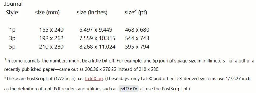
The designations 1p, 3p, and 5p denote, respectively, Elsevier’s standard journal styles, which are officially called 1+, 3+ and 5+. In particular, each style has a distinct paper size (the same size for both printed and pdf versions).

Here is a visual comparison of the three formats, using actual pages from recently published papers (as of Dec. 2020):

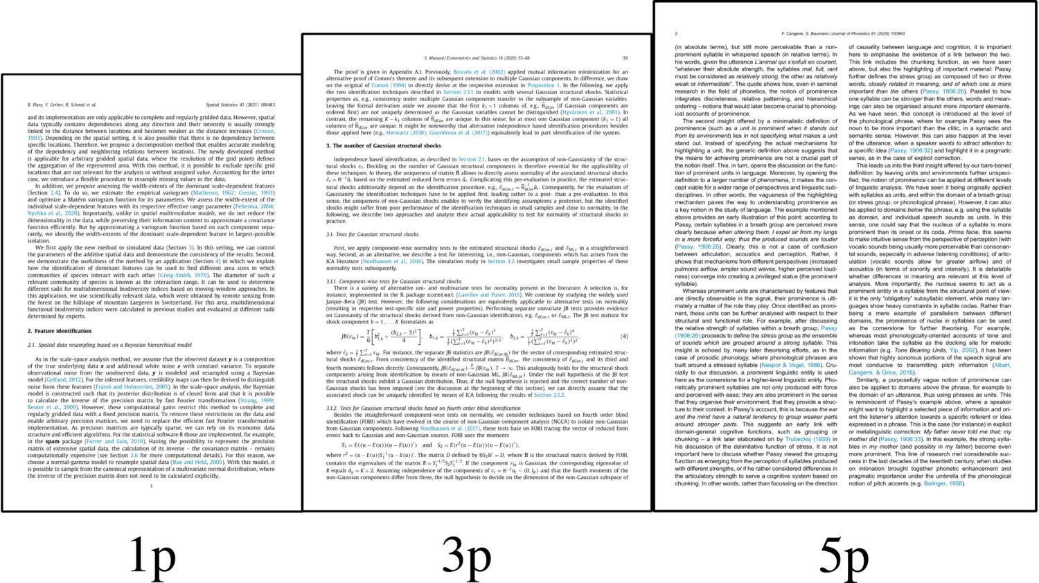
The sizes are as follows:

Feature scaling

Rescaling (min-max normalization)

x'=\frac{x-\min(x)}{\max(x)-\min(x)}

To rescale a range between an arbitrary set of values [a, b], the formula becomes:

x'=a+\frac{(x-\min(x))(b-a)}{\max(x)-\min(x)}

Mean normalization

x'=\frac{x-\bar{x}}{\max(x)-\min(x)}

Standardization (Z-score Normalization)

x'=\frac {x-{\bar {x}}}{\sigma }

where \sigma is standardeviation.

Robust Scaling

x'=\frac {x-Q_{2}(x)}{Q_{3}(x)-Q_{1}(x)}

where Q_1(x), Q_2(x), Q_3(x) are the three quartiles (25th, 50th, 75th percentile).